Gaussian Process Tutorial

This is the first part of a two-part blog post on Gaussian processes. If you would like to skip this overview and go straight to making money with Gaussian processes, jump ahead to the second part.

In this post, I’ll provide a quick tutorial on using Gaussian processes for regression, mainly to prepare for a post on one of my favorite applications: betting on political data on the website PredictIt. This post is intended for anyone who has taken an intro probability class and has basic machine learning experience, as my main goal is to provide intuition for Gaussian processes. Thus, it is not meant to be exhaustive at all. Be sure to check out Carl Rasmussen and Christopher Williams’s excellent textbook Gaussian Processes for Machine Learning (available for free online) for a more comprehensive reference.

Gaussian Process Tutorial

What is a Gaussian process? Frequently, it is referred to as the infinite-dimensional extension of the multivariate normal distribution. This may be confusing, because we typically don’t observe random variables with infinitely many components. However, when we work with GPs, the intuition is that we observe some finite-dimensional subset of infinite-dimensional data, and this finite subset follows a multivariate normal distribution, as would every finite subset.

For example, suppose we measure the temperature every day of the year at noon, resulting in a 365-dimensional vector. In reality, temperature is a continuous process, and the choice to take a measurement every day at noon is arbitrary. What would happen if we took the temperature in the evening instead? What if we took measurements every hour or every week? If we model the data with a GP, we are assuming that each of these possible data collection schemes would yield data from a multivariate normal distribution.

Thus, it makes sense to think of a GP as a function. Formally, a function \(\boldsymbol f\) is a GP if any finite set of values \(f(\boldsymbol x_1), \dots, f(\boldsymbol x_n)\) has a multivariate normal distribution, where the inputs \(\{\boldsymbol x_n\}_{n=1}^N\) correspond to objects (typically vectors) from any arbitrarily sized domain. For example, in the temperature example, \(\{\boldsymbol x_n\}_{n=1}^{365}\) correspond to the days of the year, and \(f(\boldsymbol x_n)\) indicates the temperature measurement at day \(n\).

A GP is specified by a mean function \(m(\boldsymbol x)\) and a covariance function \(k(\boldsymbol x, \boldsymbol x')\), otherwise known as a kernel. That is, for any \(x, x'\), \(m(\boldsymbol x) = \mathbb E[f(\boldsymbol x)]\) and \(k(\boldsymbol x, \boldsymbol x') = \text{Cov}(f(\boldsymbol x),f \boldsymbol (x'))\). The shape and smoothness of our function is determined by the covariance function, as it controls the correlation between all pairs of output values. Thus, if \(k(\boldsymbol x, \boldsymbol x')\) is large when \(\boldsymbol x\) and \(\boldsymbol x'\) are near one another, the function will be more smooth, while smaller kernel values imply a more jagged function.

Given a mean function and a kernel, we can sample from any GP. Say we want to evaluate the function at \(N\) inputs, each of which has dimension \(D\). We first create a matrix \(\boldsymbol X \in \mathbb{R}^{N \times D}\), where each row corresponds to an input we would like to sample from. We then evaluate the mean function at all inputs, denoted by \(\boldsymbol{m}_{\boldsymbol X}\) (a vector of length \(N\)), and the kernel matrix corresponding to \(\boldsymbol X\), denoted by \(\boldsymbol K_{\boldsymbol X \boldsymbol X}\), defined by

More generally, for any two sets of input data, \(\boldsymbol X\) and \(\boldsymbol X'\), we define \(\boldsymbol K_{\boldsymbol X \boldsymbol X'}\) to be the matrix where the \((i,j)\) element is \(k(\boldsymbol x_i, \boldsymbol x_j')\). Finally, we can sample a random vector \(\boldsymbol f\) from a multivariate normal distribution: \(\boldsymbol f \sim \mathcal N(\boldsymbol m_{\boldsymbol X}, \boldsymbol K_{\boldsymbol X \boldsymbol X})\). By construction, \(\mathbb E(f(\boldsymbol x_n)) = m(\boldsymbol x_n)\) for all \(n\) and \(\text{Cov}(f(\boldsymbol x_n), f(\boldsymbol x_m)) = k(\boldsymbol x_n, \boldsymbol x_m)\) for all pairs \(n,m\). Because this vector has a multivariate normal distribution, all subsets also follow a multivariate distribution, fulfilling the definition of a GP.

Choosing an appropriate kernel may not be a straightforward task. The only requirement is that the kernel be a positive-definite function that maps two inputs, \(\boldsymbol x\) and \(\boldsymbol x'\), to a scalar, so that \(\boldsymbol K_{\boldsymbol X \boldsymbol X}\) is a valid covariance matrix. Thus, it is typical to choose a kernel that can approximate a large variety of functions. I won’t go over different types of kernels here, but the kernel cookbook by David Duvenaud provides a great overview of popular kernels for GPs.

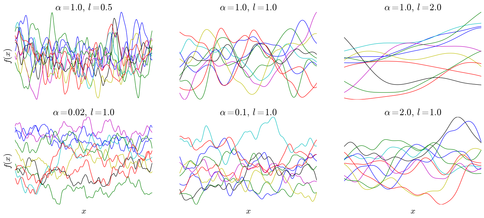
For example, consider single-dimensional inputs \(\{x_n\}\) with a constant mean function at 0 and the following kernel:

where \(k, \alpha,\) and \(l\) are all positive real numbers, referred to as hyper-parameters. This is known as the rational quadratic covariance function (RQ). I won’t go into much detail about this particular kernel, but note that it only depends on the inputs via their difference \((x-x')\), meaning the shape of the function is constant throughout the input space. Additionally, as \(x\) and \(x'\) are closer to one another, the covariance is larger, resulting in continuity. Below are samples drawn from a GP with a rational quadratic kernel and various kernel parameters, with \(h\) fixed at 1:

Note that after importing numpy and defining the RQ covariance, these plots are easily generated with three lines in Python:

    plot_xs = np.reshape(np.linspace(-5, 5, 300), (300,1))
    sampled_funcs = np.random.multivariate_normal(np.ones(len(plot_xs)), rq_covariance(params,plot_xs,plot_xs), \
                        size=10)
    ax.plot(plot_xs, sampled_funcs.T)

The complete code used to generate these plots is available here.

Typically, we would like to estimate function values of a GP conditioned on some training data, rather than merely sample functions. We are typically given a set of inputs \(\boldsymbol X \in \mathbb{R}^{N \times D}\) and corresponding outputs \(\boldsymbol f \in \mathbb{R}^n\), and we would like to estimate the outputs \(\boldsymbol f_*\) for a set of new inputs \(\boldsymbol X_*\). In the simplest, noise-free case, we can model \(\boldsymbol f\) as a GP. What does this mean? We have observed data \((\boldsymbol f)\) and unobserved data \((\boldsymbol f_*)\) coming from a GP, so we know that concatenating \(\boldsymbol f\) and \(\boldsymbol f_*\) results in a multivariate normal with the following mean and covariance structure:

If this notation is unfamiliar, we’re just concatenating vectors and matrices. For example, the mean parameter of this multivariate normal is \(\boldsymbol m_{\boldsymbol X}\) concatenated with \(\boldsymbol m_{\boldsymbol X_*}\).

Now, because \(\boldsymbol f\) is observed, we can model \(\boldsymbol f_*\) using the conditional distribution of a multivariate normal, given by:

This is a known result of the multivariate normal distribution; if this is result is unfamiliar, this Stack Exchange answer gives a pretty neat derivation. Thus, we not only have an estimate of function values, but we also have complete knowledge of the predictive covariance in closed form, making it possible to assess uncertainty. This will come in handy for betting on political data.

A subtle note is that typically we do not have access to the function values themselves, but rather noisy observations \(y_n = f(\boldsymbol x_n) + \epsilon_n\) where \(\epsilon_n \sim \mathcal N(0, \sigma^2_\epsilon)\) i.i.d. We can incorporate this noise into our model by adding \(\sigma_\epsilon^2\) to every diagonal term in \(\boldsymbol K_{\boldsymbol X \boldsymbol X}\), which corresponds to an updated kernel.

Thus, we can make predictions and compute their uncertainty in closed form. How do we choose the hyper-parameters \(\boldsymbol \theta\) (which consists of \(h,\alpha,l,\) and \(\sigma^2_{\epsilon}\) in the case of the RQ covariance)? Recall that we are assuming \(\boldsymbol y \sim \mathcal{N}(\boldsymbol m_{\boldsymbol X}, \boldsymbol K_{\boldsymbol X \boldsymbol X})\), so the marginal likelihood of the data \(p(\boldsymbol y \vert \boldsymbol X, \boldsymbol \theta)\) is the multivariate normal density. Thus, we can choose our hyper-parameters by setting them to the values that maximize the marginal likelihood (or, more easily, the log marginal likelihood, as log is monotonic) with respect to \(\boldsymbol \theta\). We can do this with black-box optimizers in Python or R.

Rasmussen and Williams show that the likelihood incorporates a tradeoff between fit and model complexity, so overfitting tends to be less significant a problem in GP regression. A downside, however, is that every iteration of optimization requires the inversion of an \(N \times N\) matrix, which is \(\mathcal O(N^3)\).

Now that we’re all experts on GPs, head to the second part of this blog post to learn how to make money with GPs.