The Box-Muller Transform

Every statistician has a favorite way of generating samples from a distribution (not sure if I need a citation for this one). From rejection sampling to Hamiltonian Monte Carlo, there are countless methods to choose from (my personal favorite is rnorm).

One of the most interesting and counterintuitive sampling techniques is the Box-Muller transform. I’m not sure how widely it’s used today, but given two samples from a uniform distribution, it can generate two independent samples from a standard normal distribution.

The idea behind the Box-Muller transform is to imagine two independent samples \(X, Y \sim \mathcal{N}(0,1)\) plotted in the Cartesian plane, and then represent these points as polar coordinates. Recall, to transform to polar, we need the distance \(R\) between \((X,Y)\) and the origin along with \(\theta\), the angle this line segment makes with the x-axis.

We start with the distance from the origin, \(R = \sqrt{X^2 + Y^2}\). For simplicity, we work with \(R^2 = X^2 + Y^2\). The sum of two independent squared standard normals follows a chi-squared distribution with 2 degrees of freedom. It is also a known fact that a chi-squared distribution with 2 degrees of freedom is equivalent to a \(\text{Gamma}(1,\frac{1}{2})\) random variable, which is itself equivalent to a \(\text{Expo}(\frac{1}{2})\) variable. Finally, we can express an exponential random variable as the log of a uniform. More succinctly,

where \(U_1 \sim \text{Unif}(0,1).\)

What about the angle, \(\theta\)? If we write the joint density of \(X\) and \(Y\), we can see

Thus, once we have \(R^2\), the squared distance between \((X,Y)\) and the origin, the joint distribution of \(X\) and \(Y\) is uniform. That is, as long as \((X,Y)\) is a pair satisfying \(X^2 + Y^2 = R^2\), it can be any point on the circle with radius \(R\). As a result, we can simply take \(\theta = 2\pi U_2\), where \(U_2 \sim \text{Unif}(0,1).\)

Putting all these results together, if we take \(R = \sqrt{-2\log U_1}\) and \(\theta = 2\pi U_2\) for \(U_1, U_2 \sim \text{Unif}(0,1)\), we have the polar coordinates for two independent standard normal draws. Thus, converting back to Cartesian, we have

This is straightforward to implement in R:

nsims = 10000
samples = rep(NA,nsims*2)
for (sim in 1:nsims) {
  us = runif(2)
  R = sqrt(-2*log(us[1]))
  theta = 2*pi*us[2]
  samples[2*sim] = R*cos(theta)
  samples[2*sim-1] = R*sin(theta) 
}

Using the above code, I compared the histogram of Box-Muller samples to those using rnorm, which were nearly identical:

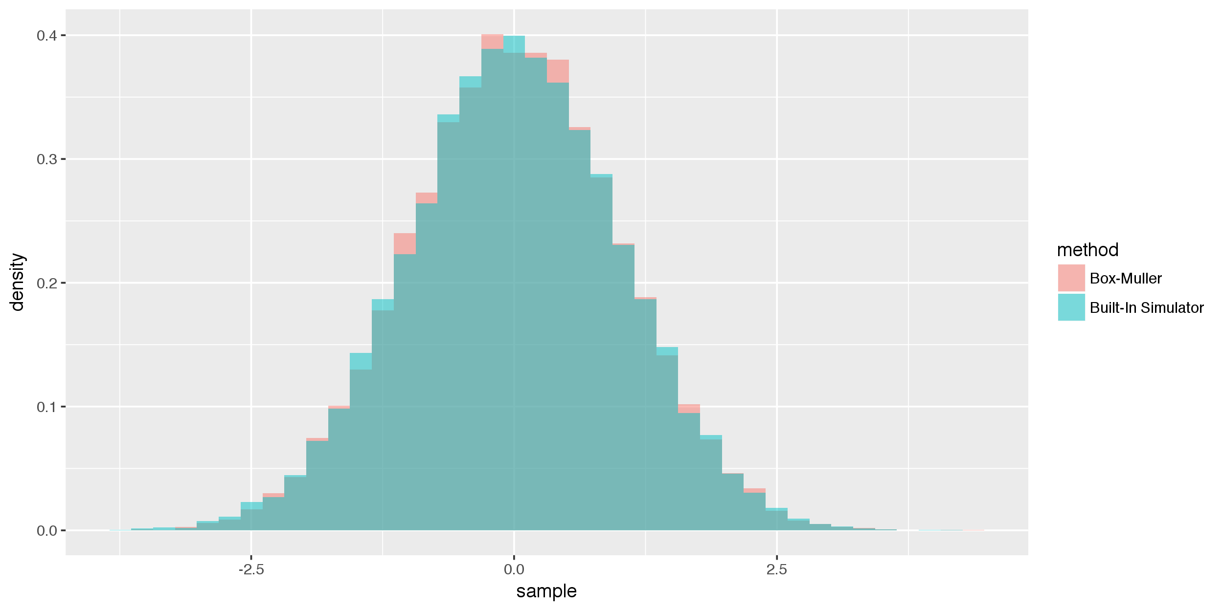
Interesting, but this is nothing more than a cool sampling trick, right? Wrong. If we represent normal random variables in Box-Muller form, it can become easier to prove results about the normal distribution.

For example, consider the problem of proving that for independent draws \(X,Y \sim \mathcal{N}(0,1)\), \(X+Y\) is independent of \(X-Y\), and both distributed as \(\mathcal{N}(0,2)\). A proof that doesn’t require the use of pdfs involves representing \(X\) and \(Y\) in Box-Muller form (I first saw this solution in Joe Blitzstein’s class Stat 210, which I encourage any Harvard student who’s reading this to take). Let \(R^2 \sim \chi^2_{df=2}\) and \(U \sim \text{Unif}(0,1)\), as in the representation above. Thus, \(X = R\cos(\theta) = R\cos(2\pi U)\), and \(Y = R\sin(\theta) = R\sin(2\pi U)\). This form gives us

Note that we use the trigonometric identities for \(\cos(\alpha + \beta)\) and \(\sin(\alpha + \beta)\) in the derivation. The final form should look familiar – we’ve recovered the Box-Muller representation, albeit with some modifications. The \(\sqrt{2}\) in front scales the standard normal so it now has a variance of 2. Additionally, note that we are using \(2\pi U + \pi/4\) as \(\theta\) instead of \(2\pi U\). However, we do not have to worry about it as it still results in a uniform sample over the possible angles.

Thus, \(X+Y\) and \(X-Y\) are independent draws from the distribution \(\mathcal{N}(0,2)\).