Betting on Politics with Gaussian Processes

This is the second part of a two-part blog post on Gaussian processes. If you would like an overview of Gaussian processes, head over to the first part.

Betting on PredictIt with Gaussian Processes

One of my favorite websites is PredictIt, which provides prediction markets for betting on politics. Many of these markets are not explicitly quantitative, such as Will there be a Putin-Trump meeting in U.S. in Trump’s first 100 days?. However, certain markets involve predicting polling numbers or election winners, which are possible to model with machine learning techniques.

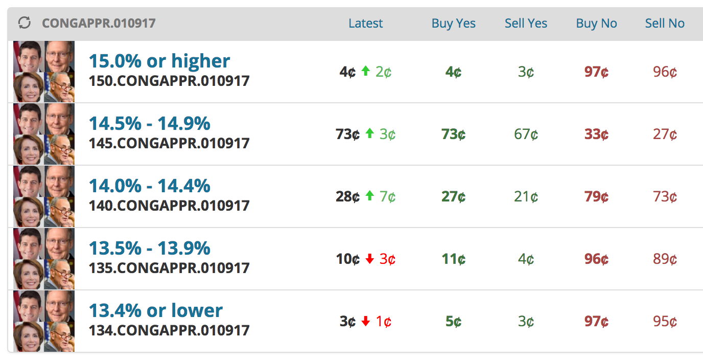
In this post, I’m going to focus on the market What will congressional job approval be on January 9? (today is January 4). The congressional job approval is taken from a polling average aggregated on the website RealClearPolitics, which averages polls from Gallup, Monmouth, and Economist/YouGov, among others. There are five possible buckets for the average job approval on January 9, and users can either “Buy Yes” or “Buy No” on each outcome.

In all cases, we are rewarded with $1.00 per share for accurate estimates. For example, in the screenshot above, we can “Buy Yes” for “14.0% - 14.4%” for $0.27. We will then receive a net profit of $0.73 if the average congressional job approval is between 14.0% and 14.4% on January 9, and we will lose our $0.27 otherwise. Thus, if we believe that the probability of the job approval being in this range is larger than 27%, we should buy this share. Similarly, we can “Buy No” for $0.79, and if the job approval is not in this range we will be rewarded with $0.21.

In R, I scraped the past 1,000 days of approval data from the RealClearPolitics website. I then trained a GP on these data points, which allowed me to not only make predictions for the average job approval for January 9, but also use the predictive variance to assess the uncertainty of these estimates. This made it possible to calculate the probability of being in any of the five buckets on PredictIt. Thus, if one of my predictions is significantly different from any of the market values, I would be wise to buy shares and make $$$ (assuming, of course, that this model is correct).

A few words of caution before proceeding: this model is not correct. There are many possible ways to model time series data, and a GP is just one of them. Any model that can generate predictions and uncertainty estimates would be exciting to try, and I used a GP because it’s one of my favorite models. Additionally, we are trying to model polling averages, so treating each poll individually should provide more fruitful estimates. Finally, the prices on PredictIt reflect more knowledge than simply the past 1,000 days; they take into account current events, such as whether Congress just did something unpopular (such as trying to remove an ethics committee), and the schedule of poll releases. Our model uses only prior data, so somehow accounting for these factors would make it more robust.

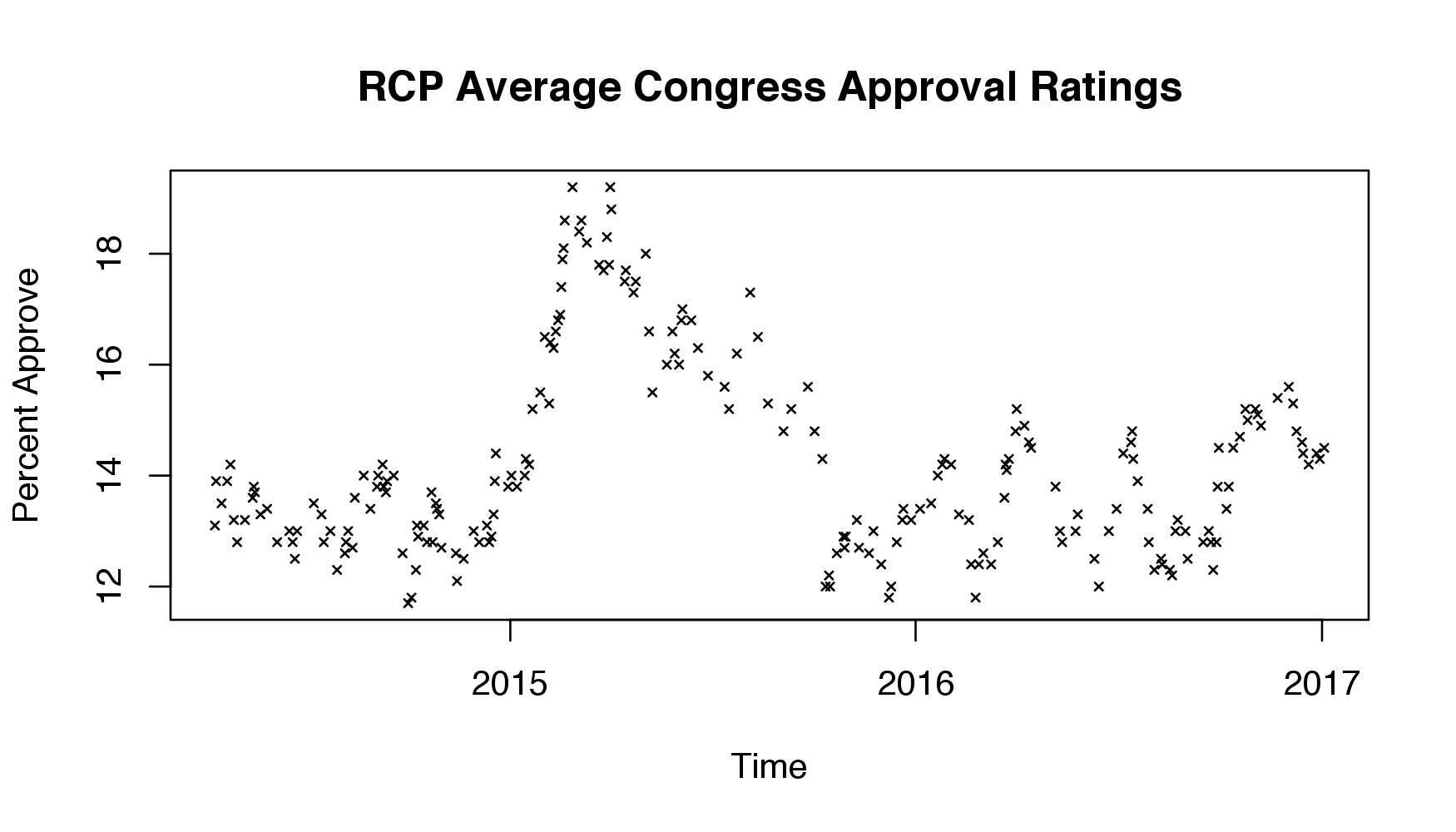
Once I scraped the data, I removed consecutive days where the average didn’t change. I did this becuase there are some days where no new polls are added to the aggregate, so I removed them instead of accounting for these days in the model. The data is below:

I chose to use a constant mean function and the rational quadratic covariance function (RQ) as my kernel. This is an area where the model can be significantly improved: I would imagine it’s more appropriate to use some combination of kernels, especially if there is a linear or periodic effect. However, the RQ kernel appeared to provide sensible results, so I stuck with it.

I then used R’s optim command to optimize the log-likelihood \(p(\boldsymbol y \vert \boldsymbol X, \boldsymbol \theta)\) where \(\boldsymbol y\) is the polling data averages, \(\boldsymbol X\) consists of the days corresponding to the polling data, and \(\boldsymbol \theta\) are the RQ hyper-parameters along with the noise-scale \(\sigma^2_{\epsilon}\) and the constant mean parameter. Because some of these parameters were constrained to be positive, I parameterized them by their log when optimizing.

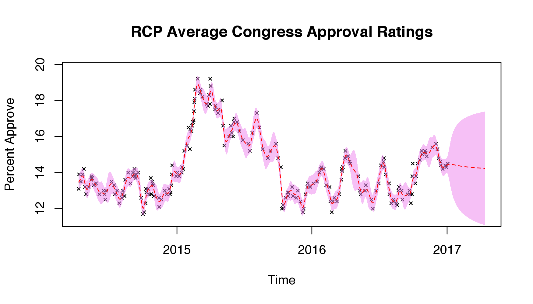
After choosing my hyper-parameters, I calculated the predictive mean for the past 1,000 days and the next 100 along with the 95% confidence interval using the predictive covariance:

The dashed red line represents the predictive mean at each time point, and the shaded purple represents the 95% confidence interval. As we can see, the data fits nicely, and, as desired, the uncertainty of the estimates increases as we move away from the data and model the next 100 days. If anything, there appears to be a slight downward trend as we head into the future, perhaps reflecting that most recently, the approval ratings have been decreasing.

Finally, I calculated my estimates for each PredictIt bucket for January 9:

\begin{array}{c|cccc} \text{Approval Rating} & \text{“Yes” Price} & \text{Model “Yes” Probability} & \text{“No” Price} & \text{Model “No” Probability} \
\hline\text{15.0% or higher} & $0.04 & 20\% & $0.97 & 80\%\
\text{14.5% - 14.9%} & $0.75 & 31\% & $0.33 & 69\%\
\text{14.0% - 14.4%} & $0.27 & 30\% & $0.79 & 70\%\
\text{13.5% - 13.9%} & $0.11 & 14\% & $0.96 & 86\%\
\text{13.4% or lower} & $0.03 & 4\% & $0.97 & 96\%\
\end{array}

Thus, the most under-valued markets are buying “Yes” for “15.0% or higher” ($0.04 for 20%) and buying “No” for “14.5% - 14.9%” ($0.33 for 69%). The remaining markets more-or-less align.

I find it interesting that the “Yes” price is so high for “14.5% - 14.9%” compared to my model. The most recent polling average was 14.5 for January 3, which is right on the border of the second and third buckets (recall we’re trying to make estimates for January 9). My guess is that this reflects some outside knowledge such as no polls being conducted in the next 5 days.

Regardless, I bought 50 shares of “Yes” for “15.0% or higher” (for a total of $2.00) and 12 shares of “No” for “14.5% - 14.9” (for a total of $3.96). I’ll be sure to provide updates with how much money I win/lose. I’d love to try out more elaborate kernels or even a deep Gaussian Process in future posts and see how these models fare.

All my code is available here.

Update

I didn’t make any money with these shares – as I predicted, RCP didn’t add any more polls to the aggregate average. In the future, I’ll tweak this model and hopefully find ways to account for the timing of polls. Stay tuned!