Is the Hot Hand Fallacy a Fallacy?

In this post, I’m going to delve into a result from the paper Surprised by the Gambler’s and Hot Hand Fallacies? A Truth in the Law of Small Numbers by Joshua Miller and Adam Sanjurjo. The paper covers a really counterintuitive result, so I recommend checking it out.

The Hot Hand Fallacy

In basketball, there is a belief among players that if someone goes on a streak and makes a series of consecutive shots, they are more likely to make their next shot. This belief was discussed and debunked in a landmark paper by Gilovich, Vallone, and Tversky, The Hot Hand in Basketball: On the Misperception of Random Sequences, leading to the term “hot hand fallacy” (by the way, this is the same Tversky who is profiled in Michael Lewis’s excellent new book, The Undoing Project).

However, since the original publication in 1985, this result has been challenged numerous times, and, as far as I can tell, there still isn’t a common consensus on whether the hot hand exists. Most recently, Miller and Sanjurjo have argued that the original paper missed a key mathematical bias that, when accounted for, would imply the existence of the hot hand. They conclude:

“Because researchers have: (1) accepted the null hypothesis that players have a fixed probability of success, and (2) treated the mere belief in the hot hand as a cognitive illusion, the hot hand fallacy itself can be viewed as a fallacy.”

I won’t attempt to answer whether the hot hand exists, but I did want to go over the counterintuitive result from Miller and Sanjurjo. They begin with a thought experiment. Say we flip a fair coin 100 times, and we would like to know the outcome that typically follows heads. So, whenever we flip a head, we get our pen and paper ready and write down the result of the following flip.

Question: What is the expected proportion of heads written on this piece of paper? Obviously one-half, right?

Answer: Less than one-half.

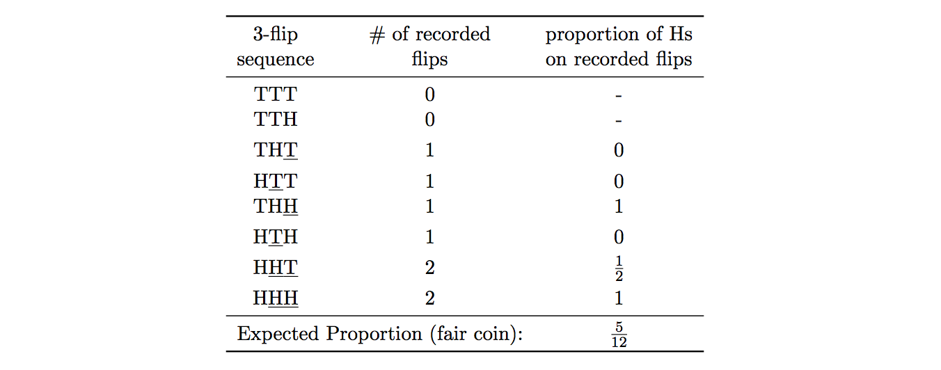
Counterintuitive, right? They walk through the result for 3 flips, showing the expected proportion of heads is \(\frac{5}{12}\) (this screenshot is taken from the paper):

We can see how this bias applies to basketball – instead of coin tosses, we are dealing with basketball shot attempts. It turns out this generalizes to streaks longer than 1 as well (i.e. recording the result after \(k > 1\) consecutive successes) and to probabilities of success \(p \neq .5\).

In fact, we can simulate this in a few lines in R. Setting nsims = 5000, n = 100, p = .5, we can use:

results = rep(NA,nsims)
for (sim in 1:nsims) {
  tosses = rbinom(n,1,p)
  candidates = which(tosses == 1) + 1
  observed_candidates = candidates[candidates <= n]
  results[sim] = sum(tosses[observed_candidates])/length(observed_candidates)
}
expected_heads = mean(na.omit(results))

Running this code, I get expected_heads = .494, so sligtly less than half. Setting n = 3, we can verify expected_heads = .415, so right around \(\frac{5}{12} \approx .417\).

We can also vary streak lengths and probabilites of success in R for different values of \(n\), corresponding to the length of the sequence. Here are my results for probabilities of success \(p\) = 0.25, 0.50, 0.75 and streak lengths of \(k\) = 1, 2, and 3, using 5,000 simulations (for the first graph, I used a fix streak of length \(k\) = 1, and for the second, I used a fix probability of \(p\) = 0.50):

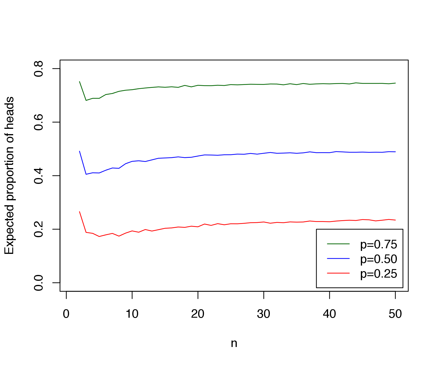
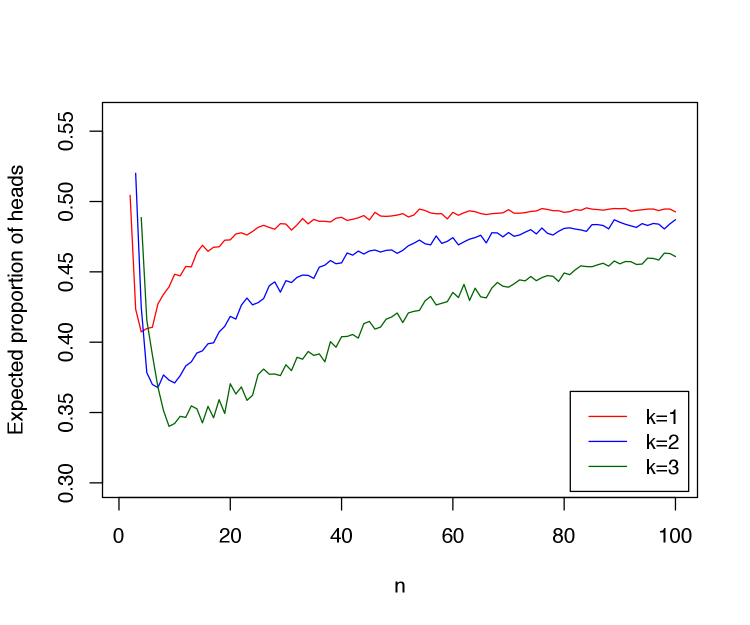
As we can see, the bias exists for multiple values of \(p\), and it actually grows with the streak length \(k\). Therefore, applying this bias to basketball, if researchers only note the shots taken after \(k = 3\) (or something) successes, they must account that mathematically, the expected probability of success is lower than \(p\), that player’s typical shooting percentage. So, if they don’t account for this bias, they may come to the conclusion that a player is shooting worse than he actually is, which may result in ignoring a hot hand effect if there happens to be one. Miller and Sanjurjo conclude that there is indeed a hot hand effect, which went unnoticed by Gilovich, Vallone, and Tversky because they did not account for this bias.

Miller and Sanjurjo mathematically derive the bias in general settings, but the math is a little hairy. Here’s a brief intuition. Suppose that we have a sequence of Bernoulli\((p)\) random variables \(\boldsymbol X = \{X_i\}_{i=1}^n\), and we want to estimate the probability of success for trial \(t\) given that \(t\) follows \(k\) consecutive successes.

Suppose that a researcher is looking at this data, and she decides to randomly circle one of the outcomes that follows a success. That is, if \(I(\boldsymbol X)\) is the set of indices following \(k\) successes, she randomly chooses an index \(\tau\) from this set such that \(P(\tau = t \vert \boldsymbol X) = 1/\vert I(\boldsymbol X)\vert\) for \(t \in I(\boldsymbol X)\). If we show that \(P(X_{t} = 1 \vert \tau = t)\) < \(p\), we have shown the existence of our bias.

It is easily derivable via Bayes rule that it is enough to show \(P(\tau = t \vert X_t = 0) > P(\tau = t \vert X_t = 1)\). Now, the key idea is that because we are choosing randomly from trials, when \(X_t = 1\), the set \(I(\boldsymbol X)\) is 1 element larger than it would otherwise be, meaning the probability of choosing any one index is slightly smaller. That is, because \(P(\tau = t \vert \boldsymbol X)\) is \(1/\vert I(\boldsymbol X) \vert\), when \(X_t = 1\) and every other element of \(\boldsymbol X\) is the same, \(\vert I(\boldsymbol X) \vert\) increases by 1. Therefore, \(P(\tau = t \vert X_t = 0) > P(\tau = t \vert X_t = 1)\) and \(P(X_{t} = 1 \vert \tau = t)\) < \(p\), as desired.

The code used to generate these plots is available here. I also recommend checking out the Miller and Sanjurjo paper, along with this discussion on Andrew Gelman’s blog.