Tweet Counts as Poisson GLMs

Last week, I wrote about modeling tweet counts as a simple Poisson process. In this post, I’ll dive into a slightly more sophisticated method, so check out the previous post for some background.

I’m interested in estimating the number of tweets President Trump will post in a given week so I can use the model to bet on PredictIt. My post last week demonstrated that a stationary Poisson process had some weaknesses – the rate wasn’t constant everywhere, and Trump’s tweets seemed to self-excite (i.e. if he’s in the middle of a tweet storm, he’s likely to keep tweeting).

In this post, I’ll focus on modeling tweet counts as a Poisson generalized linear model (GLM). (You probably won’t need to know much about GLMs to understand this post, but if you’re interested, the canonical text is by Peter McCullagh and John Nelder. I also highly recommend Alan Agresti’s textbook, which I used in his class.) The model will be autoregressive, as I will include the tweet counts for the previous few days among my set of predictors.

First I’ll go over the results, so jump ahead if you’re interested in the more technical model details.

Results

In short, my model uses simulations to predict the weekly tweet count probabilities. That is, it simulates 5,000 possible versions of the week, and counts how many of these simulations are in each PredictIt bucket. It uses these counts to assign probabilities to each bucket.

I ran the model last night and compared the results to the probabilities on PredictIt – all of my predictions were within three percentage points of those online, with the exception of one bucket that was eight off (the “55 or more” bucket, which my model thought was less likely than the market). Running it again this morning, however, something was off – the odds in the market had shifted considerably toward preferring less tweets, at odds with my model.

Confused, I read the comments, which indicated that seven tweets had been removed from Trump’s account this morning. However, the removed tweets were from a while ago, so I was confused why they would make a difference in this week’s count. Then I read the market rules:

“The number of total tweets posted by the Twitter account realDonaldTrump shall exceed 34,455 by the number or range identified in the question…The number by which the total tweets at expiration exceeds 34,455 may not equal the number of tweets actually posted over that time period … [since] tweets may be deleted prior to expiration of this market.”

D’oh. That didn’t seem like the smartest rule. It meant the number of weekly tweets could be negative if Trump deleted a whole bunch of tweets from before the week. There weren’t many options for modeling these purges with the data at hand. Therefore, I decided to assume that no more tweets would be deleted this week, and subtracted the 7 missing tweets from the simulation.

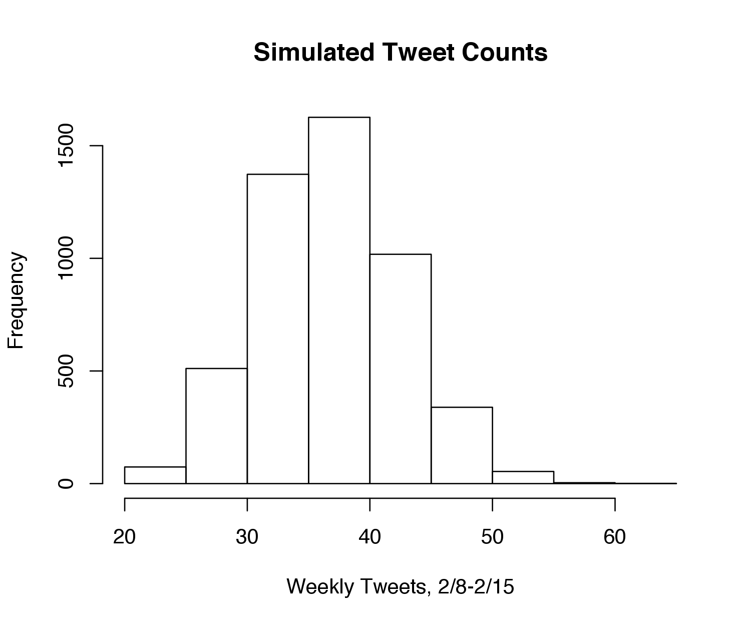
I ran the model on Friday evening, with the following histogram depicting the distribution of simulated total weekly tweet counts:

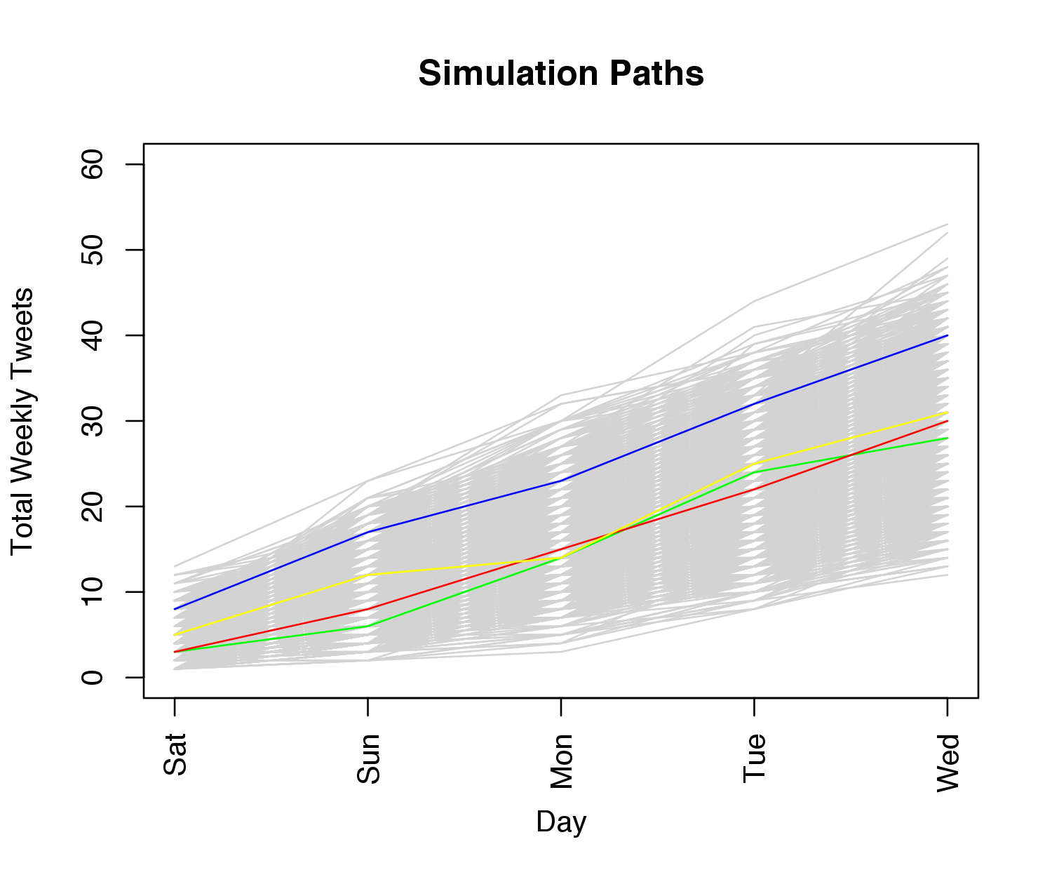
The following plot shows the simulated trajectories for the week, with 4 paths randomly colored for emphasis:

Finally, the following table shows my model probabilities, compared to those on PredictIt as of this writing:

\begin{array}{c|cccc} \text{Number of tweets} & \text{“Yes” Price} & \text{Model “Yes” Probability} & \text{“No” Price} & \text{Model “No” Probability} \
\hline\text{24 or fewer} & $0.11 & 1\% & $0.90 & 99\%\
\text{25 - 29} & $0.14 & 7\% & $0.88 & 93\%\
\text{30 - 34} & $0.23 & 24\% & $0.79 & 76\%\
\text{35 - 39} & $0.31 & 35\% & $0.73 & 65\%\
\text{40 - 44} & $0.19 & 23\% & $0.84 & 77\%\
\text{45 - 49} & $0.09 & 9\% & $0.93 & 91\%\
\text{50 - 54} & $0.05 & 2\% & $0.96 & 98\%\
\text{55 or more} & $0.04 & 0.3\% & $0.97 & 99.7\%\
\end{array}

Thus, compared to my model, the market believes Trump will have a quiet week. This may reflect the possibility of Trump deleting more tweets, or it could be some market knowledge that Trump will be preoccupied by various presidential engagements.

In general, however, the market prices align nicely with the model; no two buckets (beside the first two) disagree with the model probability by more than 4%. I think this is definitely a more robust model than the simple Poisson process, as the probabilities align quite well with the market. Thus, not expecting much in returns, I bought shares of “No” for “24 or fewer” and “25-29” and “Yes” for “35-39” and “40-44”.

Model

For this analysis, I thought it made sense to predict tweets as daily counts as opposed to weekly counts, so the predictions would be more fine-tuned. Thus, denote by \(y_t\) the number of tweets made by Trump on day \(t\). Given a vector of predictors \(\boldsymbol x_t\) for day \(t\) and a vector of (learned) coefficients \(\boldsymbol \beta\), the model I used was

Note that because we are exponentiating \(\boldsymbol x_t^T \boldsymbol\beta\), the rate parameter will never be negative, so there are no constraints on the sign of \(\boldsymbol \beta\).

To keep the model simple, I was fairly limited in my set of predictors. I included an intercept term, the day of the week, and binary variables to indicate if the tweet occurred after Trump won the election and whether the tweet occurred after the inauguration (the graph from my previous post indicates a significant changepoint after the election). I also included an indicator variable indicating whether there was a presidential or vice presidential debate – although these won’t happen again, they explain spikes in the existing data.

It also seemed reasonable that the number of Trump’s tweets today would depend on how many tweets he had in the previous few days. Thus, as a first attempt, I included the past 5 days of history, and used the following model:

Here, \(\boldsymbol x_t\) is the vector of aforementioned predictors, i.e. intercept, day of week, etc. At time \(t\), the scalars \(y_{t-1}, \dots, y_{t-5}\) indicate the counts of the previous 5 days, and each count has its own parameter to be estimated, \(\gamma_k\). Thus, this model requires that we estimate \(\boldsymbol \beta\) along with \(\gamma_1, \dots, \gamma_5\).

I used the built-in glm function in R to estimate these variables using maximum likelihood. If you’re unfamiliar with maximum likelihood, the basic idea is that we can maximize \(\sum_{t=1}^T \log p(y_t\vert x_t,y_{t-1}, \dots, y_{t-5})\) by taking the gradient with respect to our parameters \(\boldsymbol \gamma\) and \(\boldsymbol \beta\) and using an iterative method to set the gradient to 0. (I’d like to get a blog post up someday about GLMs in general so I could focus on maximum likelihood estimation and discuss some other nice properties.)

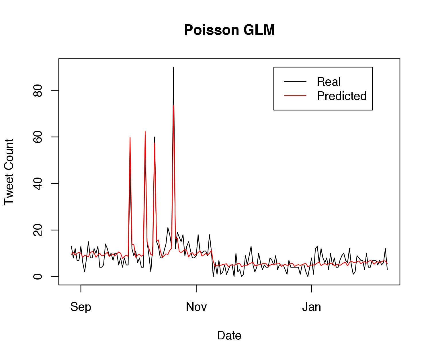
After fitting to the current data, I found that among the \(\boldsymbol\gamma\), only \(\gamma_1\) and \(\gamma_2\) were deemed statistically significant (and even these predicted values were quite small). Besides the intercept and debate indicator, the most statistically significant \(\boldsymbol\beta\) coefficient was for the indicator of being after the election, at \(-0.44\) (recall that these end up getting exponentiated). Thus, I re-ran the model using only the past two days of history (as opposed to five) in the autoregressive component. The following graph shows how the model mean fits to the training data:

Not perfect, but reasonable given the basic set of predictors, and it appears to get the general trends right. Note that the four spikes correspond exactly to the debates.

I was initially worried about overdispersion – recall that in a Poisson model, the variance of the output \(y_t\) is equal to the mean, so if the variance in reality is larger than the mean, a Poisson would be a poor approximation. Thus, I also tried using a negative binomial to model the data, which performed worse in training log-likelihood and training error. As a result, I stuck with the original Poisson model.

After estimating all the coefficients, it was time to model the probability of finishing in each bucket on PredictIt. Because the number of tweets in one day would affect the number of tweets for the next day, I couldn’t model these probabilities analytically. Thus, I ran 5,000 simulations to approximate the probability of being in each bucket by Wednesday noon.

One final note about the model – it predicts tweets for full-day length intervals, i.e. noon Monday to noon Tuesday. However, what if it’s 8 pm on Sunday, and we’re curious how often Trump will tweet before Wednesday at noon? Predicting for 2 more rows would not be enough (finishing Tuesday at 8 pm), and using 3 would be too much (finishing Wednesday at 8 pm). Thus, I decided to run an additional model that rounded at the nearest noon. That is, I duplicated the above model, except I used the number of tweets between now and the next noon as the response variable. For example, if I were running the program at 8 pm on Sunday, I would model how often Trump tweets between 8 pm and the following day’s noon for every day in the history. Then, I would use this set of coefficients to predict the tweets between now and the next noon, and then finish off all remaining full days with the coefficients from the aforementioned model. (If none of this paragraph makes sense, don’t worry about it, as it’s a pretty minor detail.)

In the future, I’d be interested in more complicated variations, such as modeling tweet deletions or using a larger set of predictors (along with performing a more rigorous dispersion analysis).

All code is available here.

Update

I bought shares in four markets (two Yes’s and two No’s). The tweet count ended up being in one of the Yes markets, good enough for a 25% return. That’s a great return, but it’s too early to say anything conclusive about the model because \(N = 1\). That being said, I’ll continue to use the GLM because the results seem promising so far.

Acknowledgments

Thanks to Scott Linderman for suggesting an autoregressive GLM model. Also thanks to Teddy Kim for various suggestions and brainstorming help. A final thank you to Owen Ward for suggesting the connection between spikes and debates in the model.