Tweet Counts as Poisson Processes

I’ve written before on using statistics to bet on PredictIt’s political markets, and this morning a new market caught my eye: How many tweets will Donald Trump post from noon Feb. 1 to noon Feb. 8?. If statistics can be used to inform any prediction market, it’s this one, so I figured I’d give this counting problem a go.

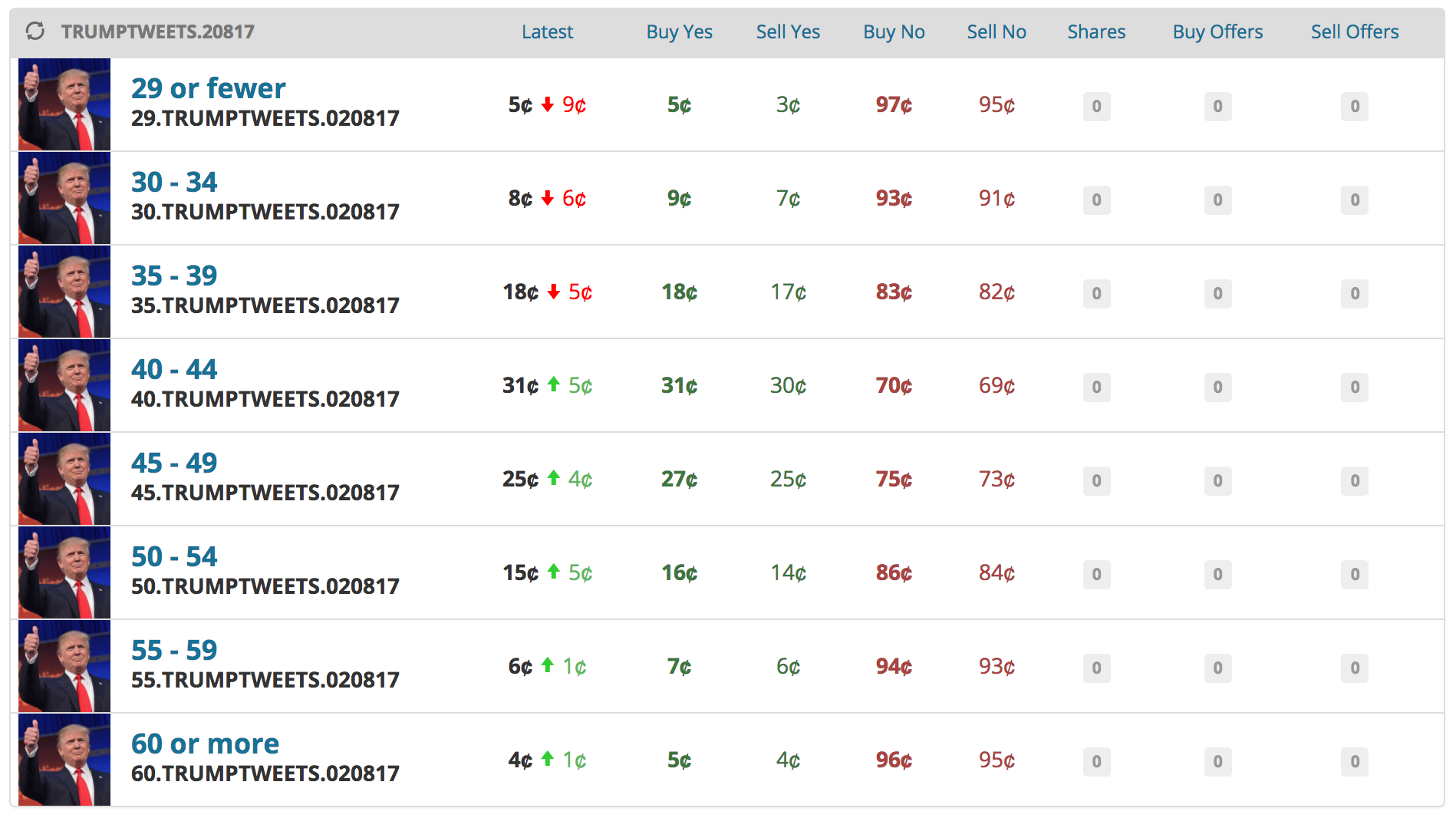
At the time of this writing, the market looked like the following: 8 buckets for the number of tweet counts, so I would need to assign a probability to each bucket:

I started by scraping Trump’s tweets on Twitter – I essentially lifted code from this tutorial by Craig Addyman. I only downloaded his last 1800 tweets, which seemed like enough because I reasoned his older tweeting habits wouldn’t be so informative nowadays.

I decided to model the number of weekly tweets as a Poisson process. For those unfamiliar with a Poisson process, the main idea is that the number of tweets \(N(t)\) in a given interval, say \([0,t)\) where \(t\) is a scalar denoting seconds, is given by a Poisson distribution with some rate \(\lambda * t\):

Moreover, this model assumes that the number of tweets in any disjoint interval is independent, and that the rate is constant for any fixed length. These assumptions are definitely wrong. There are numerous instances where Trump has rapidly strung a series of tweets together on the same topic one after another, which breaks both assumptions. Additionally, the rate is not constant, as he is much more likely to tweet during the day than during sleeping hours.

Although these assumptions are violated, I decided to use a Poisson process because it’s intuitive/straightforward (read: I’m lazy) and I didn’t have a ton of time (read: I procrastinate). Next week, I hope to use a more complicated model like a Hawkes process, so stay tuned.

The plot below shows the number of weekly tweets for all the scraped data. We can see that the stationary rate assumption is definitely violated, as it looks like his tweeting rate dropped severely after the election. As a result, I decided to only use tweet counts from after the election (even this small sample isn’t perfect, but it’s the best I could do given that there’s only been one week of presidential tweeting data).

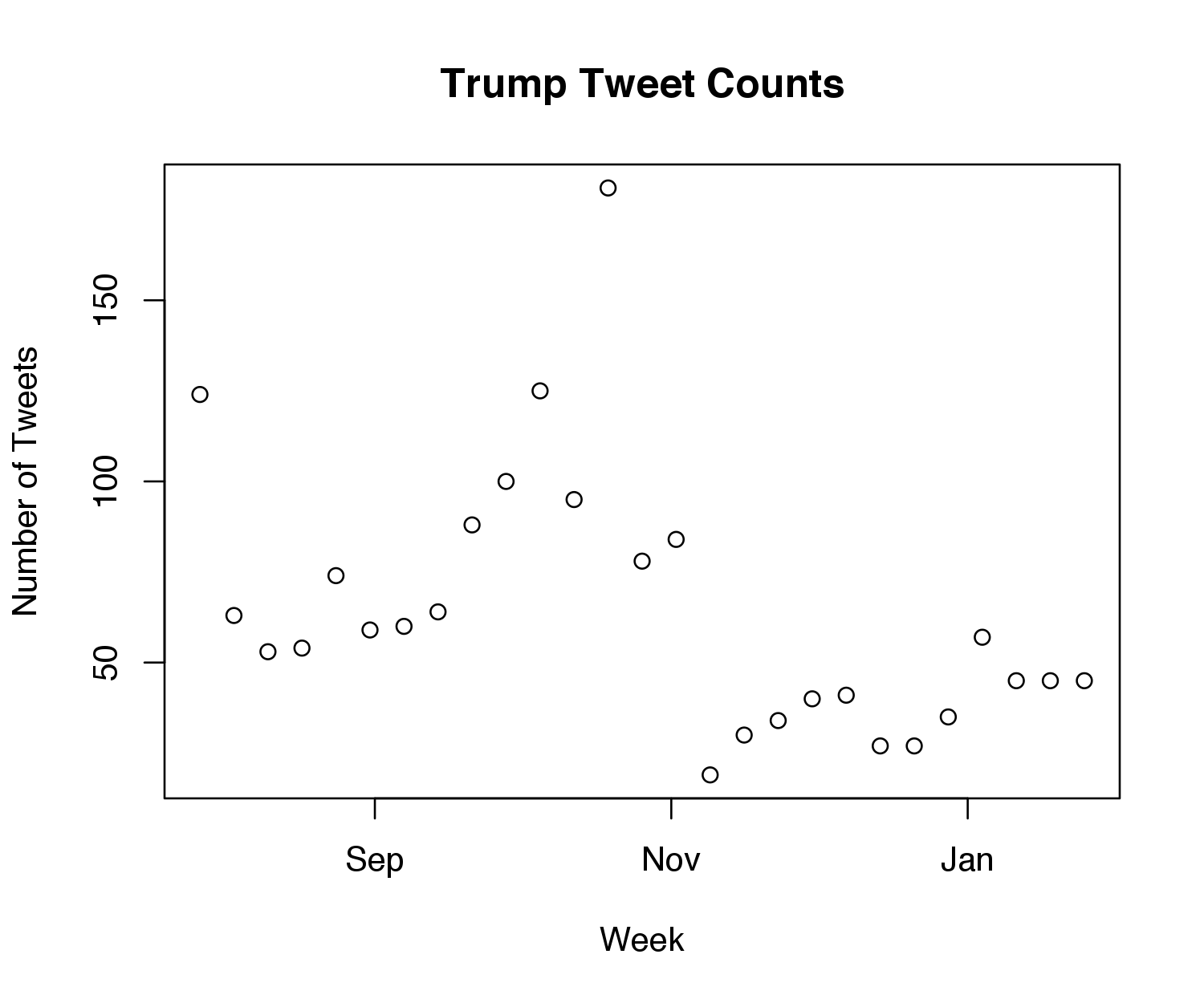
I used the maximum likelihood estimate (the average) to predict the rate, which came out to 64.7 tweets per week, or 9.24 in a day. Given the rate, I was able to put percentages on each of the buckets by taking quantiles of the Poisson distribution (after accounting, of course, for the 9 times he’s already tweeted this week).

Here are my estimates compared to their price on PredictIt:

\begin{array}{c|cccc} \text{Number of tweets} & \text{“Yes” Price} & \text{Model “Yes” Probability} & \text{“No” Price} & \text{Model “No” Probability} \
\hline\text{29 or fewer} & $0.05 & 3\% & $0.97 & 97\%\
\text{30 - 34} & $0.09 & 15\% & $0.93 & 85\%\
\text{35 - 39} & $0.18 & 33\% & $0.83 & 67\%\
\text{40 - 44} & $0.31 & 31\% & $0.70 & 69\%\
\text{45 - 49} & $0.27 & 14\% & $0.75 & 86\%\
\text{50 - 54} & $0.16 & 3\% & $0.86 & 96\%\
\text{55 - 59} & $0.07 & 0.5\% & $0.94 & 99\%\
\text{60 or more} & $0.05 & 0.04\% & $0.96 & 99.9\%\
\end{array}

It looks like my model prefers lower tweet counts since it accounts for all post-election tweets, and Trump tweeted less in November than he has done in the past few weeks. Interestingly, when I run the same model using only the last week of data to train, none of my estimates are off by more than 0.06 when compared to the market price. Therefore, it appears that the market puts more weight on his most recent tweet totals than my (admittedly basic) model.

At any rate, I decided to buy 5 shares of “Yes” for 35-39 tweets, 2 shares of “No” for 45-49 tweets, and 2 shares of “No” for 50-54 tweets (everywhere my model differed with the market prices by at least 10 percentage points). Stay tuned for updates on how I do, along with a more complicated model.

All code is available here.

Update

Trump ended up tweeting 44 times; therefore, I lost the “Yes” for 35-39 tweets, but I won both “No” markets I invested in, 45-49 and 50-54. Though it’s impossible to tell with a sample size of one, it seems like this model is a good start – Trump’s final tweet count was in the 40-44 bucket, which was deemed the second-most likely bucket by the model, at 31%.